Calibration of Photometry from WFCAM
Author: Simon Hodgkin
Document Number: VDF-TRE-IOA-00008-0010
Version Number: Draft 0.2
Date: 26th October 2005
Contents
- INTRODUCTION
- UKIDSS CALIBRATION GOALS
- MANUAL CALIBRATION
- THROUGHPUT
- RELATIVE DETECTOR SENSITIVITIES
- EXTINCTION AND NIGHT-TO-NIGHT STABILITY
- NIGHTLY CALIBRATION
- WFCAM VS UFTI
- SPATIAL SYSTEMATICS
- PIPELINE CALIBRATION
- TECHNIQUE
- CALIBRATION OF UKIRT FAINT STANDARDS
- CALIBRATION OF T DWARFS
- EXTINCTION
- 5 TOWARDS A SYSTEM OF WFCAM SECONDARY STANDARDS
- 6 SUMMARY
- Appendix A LIST OF STANDARDS
- Appendix B SYNTHETIC PHOTOMETRY
1. Introduction
I have analysed observations of standard stars and normal target
fields from semester 05A.
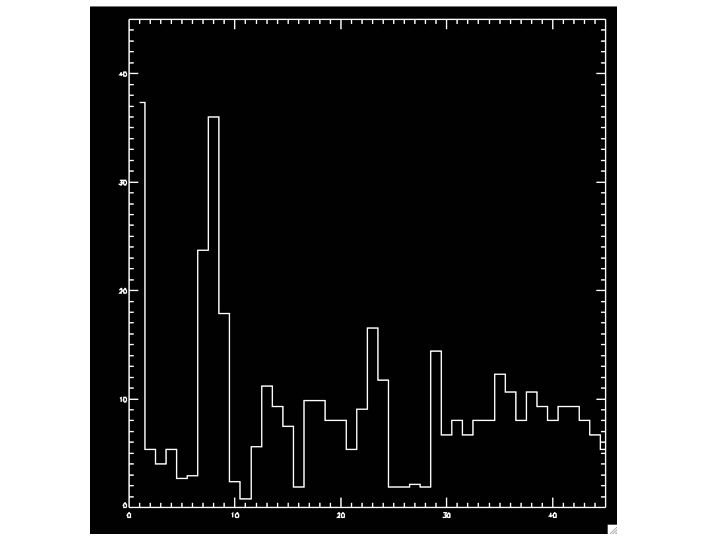 |
Figure 1: A histogram to show the number of standards
observed on each night in semester 05A. The main spike represents a
couple of nights when large numbers of standards were targetted. It
is only towards the end of the semester that observing settled into
a pattern of observing around 10 standard fields per night
(i.e. roughly hourly).
|
2. UKIDSS Calibration Goals
Requirement is photometric calibration to 2%, with a goal of 1%.
3. Manual Calibration
3.1 Throughput
The total throughput of the system is relatively easy to measure (but
much harder to quantify where in the system the actual losses are
occurring). I have assumed the following:
- The effective area of the UKIRT primary mirror is 10.5m2
(i.e. outer diameter 3.802m with an inner diameter of 1.028m). No
attempt has been made to allow for the shadowing of the primary by
the secondary, nor for any obscuration caused by the forward mounted
camera itself.
- The spectrum for Vega is interpolated over the flux values given
at the UKIRT WWW pages
(href=http://www.jach.hawaii.edu/UKIRT/astronomy/utils/conver.html)
- The filter transmissions are from Hewett et al. 2005 but
renormalized to give the relative throughput as a function of
wavelength, rather than absolute transmission (i.e. the peak value
is 1.0)
Thus the table below gives the estimated number of photons that would
be incident on the primary mirror, assuming no atmosphere, multiplied
by the relative transmission of the filter in each band. These are
converted to detector counts using an average gain of 5.1. This would
then give the zeropoint of the system in each filter if there were no
losses due to the atmosphere, telescope and the instrument. Comparison
with the measured zeropoints then give us the throughput for
WFCAM+UKIRT+atmosphere.
| Filter |
Photons
(mag=0) |
Counts
(mag=0, gain=5.1) |
ZP
(100% throughput) |
ZP
(Measured) |
Implied
Throughput |
| Z |
3.8e10 |
7.4e9 |
24.80 |
22.98 |
19% |
| Y |
3.0e10 |
5.9e9 |
24.55 |
22.81 |
20% |
| J |
2.9e10 |
5.6e9 |
24.50 |
23.00 |
25% |
| H |
3.0e10 |
5.8e9 |
24.53 |
23.24 |
30% |
| K |
1.6e10 |
3.1e9 |
23.83 |
22.55 |
31% |
Table 1: Estimate of WFCAM
throughput
Still to do: Compare to predicted throughput (Hewett et al. 2005)
3.2 Relative detector sensitivities
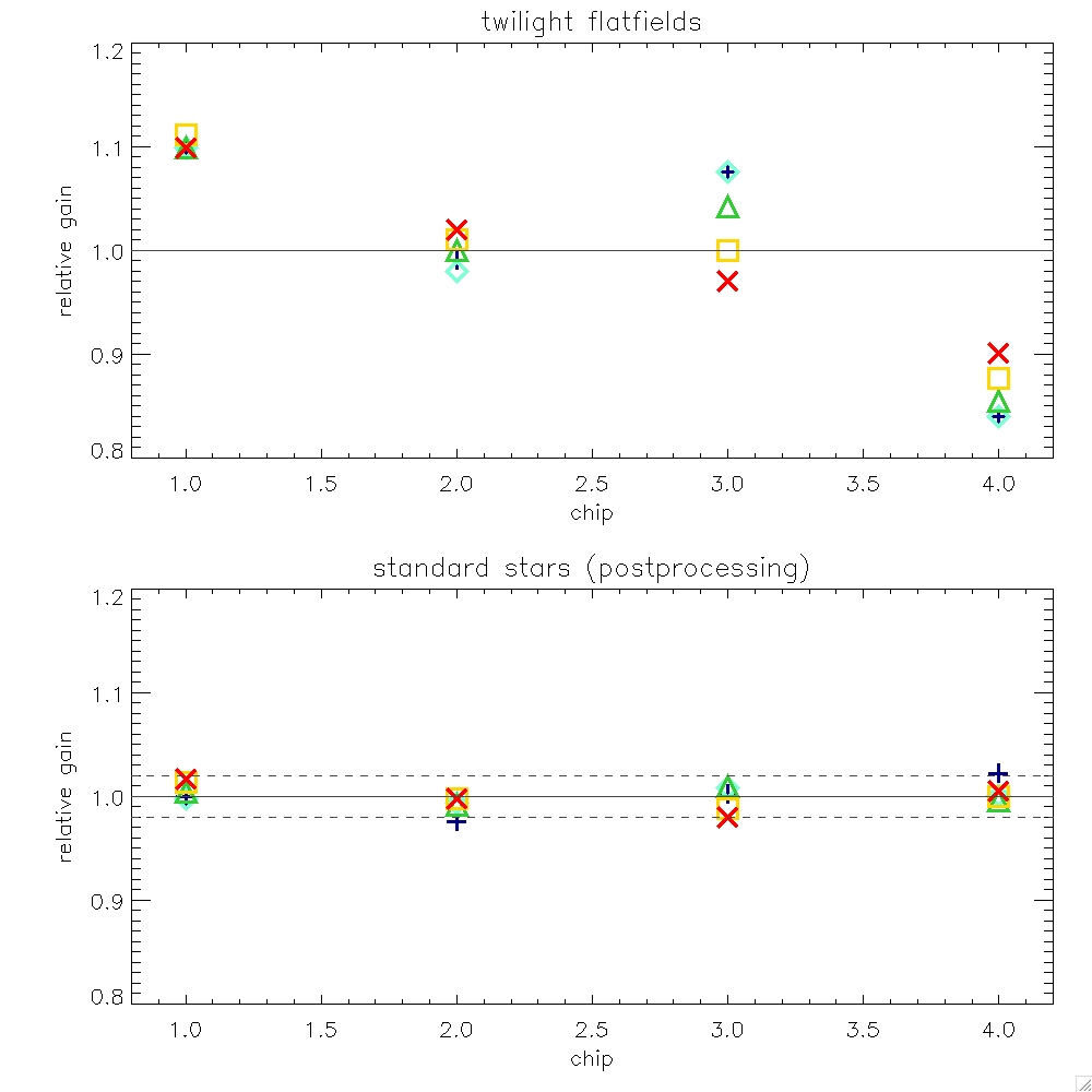
Figure 1:The top panel shows the detector-to-detector variation
in sensitivity (really it's gain*QE), measured with respect to the
mean of all 4 detectors, from twilight flatfield counts (ZYJHK). Chip
1 is the most sensitive, while chip 4 is the least. Chip 3 shows the
largest colour dependent scatter with a 10% change in relative
sensitivity between Z and K (decreasing to the red). Chip 4 shows an
increase to the red of about 8%. The bottom panel shows the
detector-to-detector gain variation measured post-pipeline processing,
i.e. the residuals after gain correction (using the twilight
flats). It is measured from the standard stars (their zeropoints). It
illustrates that the gain correction calibrates each chip to within 2%
of the mean, across all filters.
The four detectors are not uniformly sensitive. Figure 1 shows the
variation in sensitivity between the detectors as measured in the
twilight flatfields. The assumption is that the twilight sky is
flat. The detector-to-detector sensitivity is measured from the average
counts on each detector.
The ZPs derived for the night of 20050408 for each chip from the UKIRT
faint standards are summarized in Table 2.
| Filter |
chip 1 |
chip 2 |
chip 3 |
chip 4 |
|
ZP |
err |
ZP |
err |
ZP |
err |
ZP |
err |
| Z |
22.982 |
0.056 |
22.962 |
0.059 |
22.989 |
0.050 |
23.002 |
0.055 |
| Y |
22.810 |
0.018 |
22.803 |
0.016 |
22.821 |
0.015 |
22.810 |
0.020 |
| J |
23.003 |
0.021 |
22.998 |
0.020 |
23.005 |
0.026 |
23.005 |
0.021 |
| H |
23.241 |
0.017 |
23.238 |
0.016 |
23.226 |
0.019 |
23.246 |
0.014 |
| K |
22.557 |
0.016 |
22.547 |
0.021 |
22.535 |
0.021 |
22.557 |
0.016 |
Table 2: per-chip ZPs for
20050408
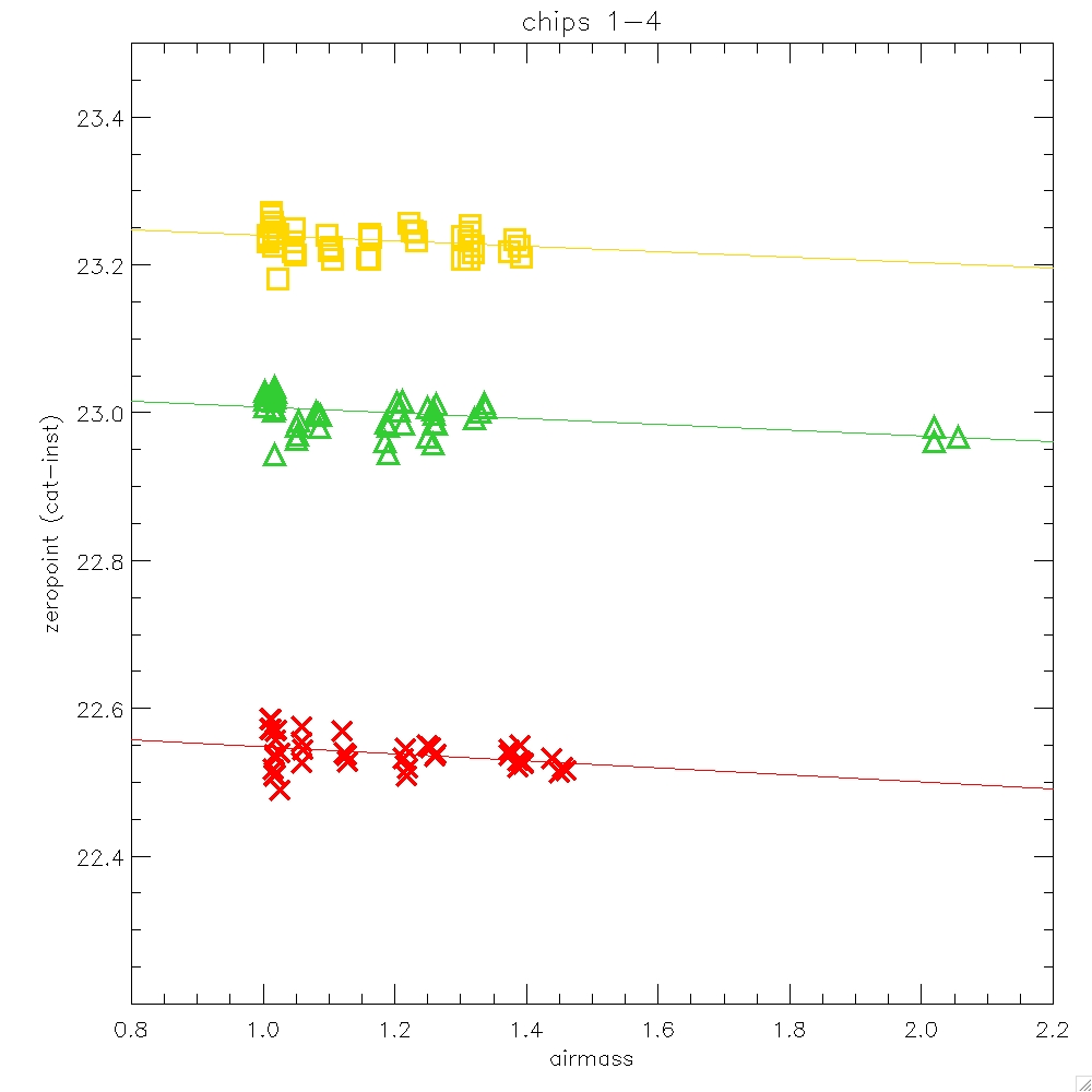
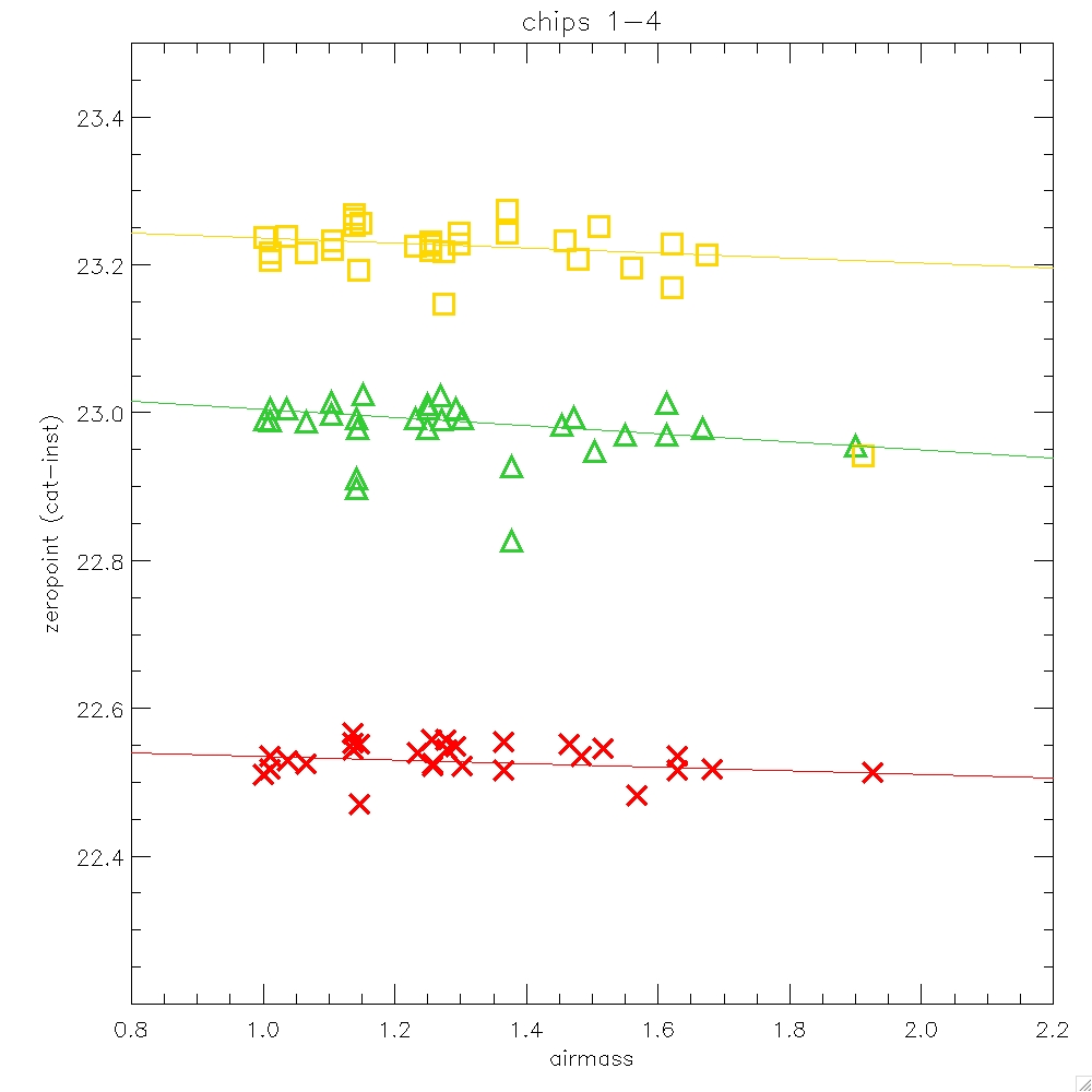
3.3 Extinction and night-to-night stability
Two nights have sufficient standards to enable a good stab at
measuring the extinction. The spread in airmass is not quite
ideal. There is coverage up to X=1.5 on April 8th and X=1.7 on April
18th. All 4 detectors are combined to constrain a fit to
mMKO – Minst = ZP – kX
with the following results:
Figure 2: Extinction diagrmas for UT20050408 and
UT20050418. All four chips have been combined onto one figure. A
better approach would be to fit the data from all four chips
simultanously, allowing ZP to vary but fixing EXT
|
20050408 |
20050418 |
| Filter |
ZP |
± |
k |
± |
ZP
| k |
| J |
23.003 |
0.015 |
0.036 |
0.012 |
23.004 |
0.055 |
| H |
23.237 |
0.024 |
0.031 |
0.021 |
23.236 |
0.033 |
| K |
22.548 |
0.024 |
0.050 |
0.020 |
22.535 |
0.024 |
Table 3: ZPs and extincxtions derived on
two nights
These values are at the lower end of site testing results. Note the
very good agreement between the ZPs derived for these two nights.
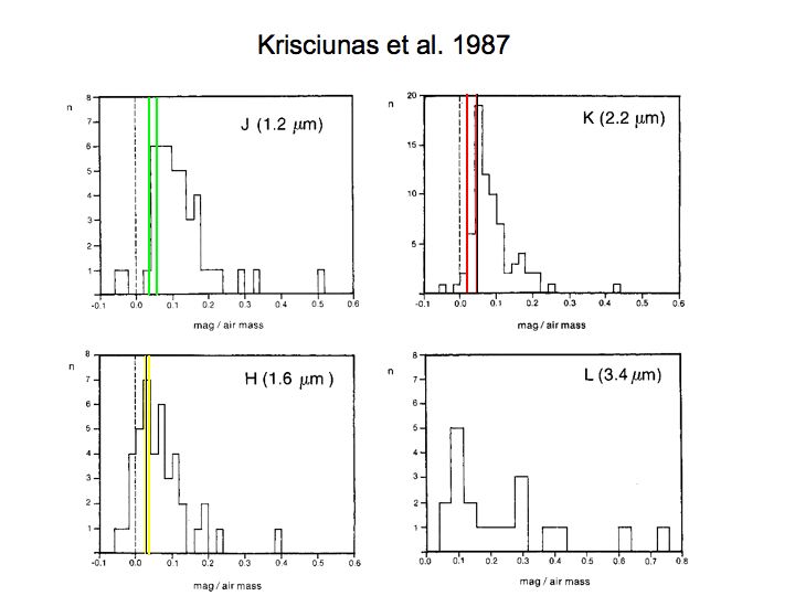
Figure 3: Figure taken from Krisciunas et al. 1987. Our
measurements overlaid
3.4 Nightly calibration
In this section I plan to discuss the calibration we hope to get on a
typical observing night. I will do this by analysing a couple of
nights where we have observed hourly standards.
3.5 WFCAM vs UFTI
Figure 4 illustrates that there is essentially no colour term between
the UFTI based UKIRT faint standard magnitudes, and the same objects
measured through the WFCAM MKO filters and detector, as expected.
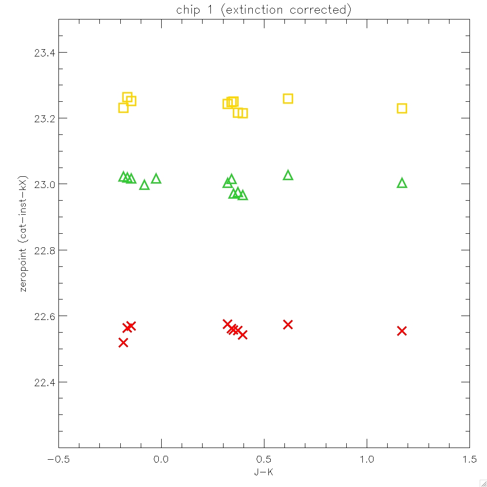
Figure 4: A plot of the offset between catalogue
magnitude and (extinction corrected) instrumental magnitude for
UKIRT faint standards on UT20050408 (JHK)
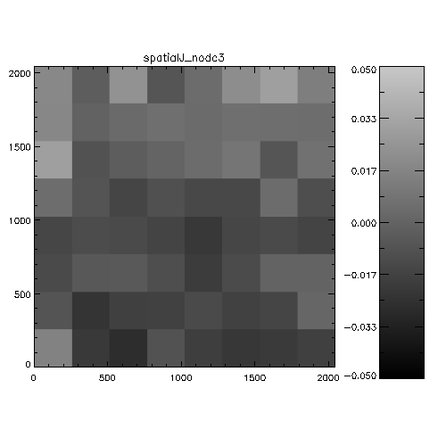
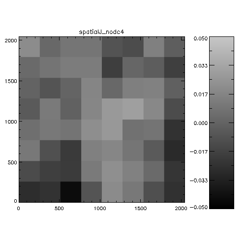
3.6 Spatial Systematics
3.6.1 From 2MASS
A simple analysis compares the WFCAM measured photometry against the
2MASS catalogue as a function of position. WFCAM sources are matched
against 2MASS. The 2MASS photometry is converted to the WFCAM system
using the colour equations listed elsewhere in this document. Only
objects brighter than J=15.5,H=15,K=15 are used, they are also
required not to be saturated in WFCAM. The offsets are combined for a
whole night and averaged over a 8x8 grid in WFCAM pixel space. Each of
these jumbo-pixels contains of order 100 stars. The rms scatter in
each jumbo-pixel is about 0.05-0.1 mags and the standard error on the
mean is about 0.005-0.01 mag. The figures below show the results for the
analysis in the J, H and K Bands.
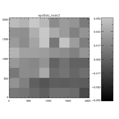
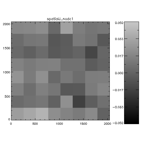
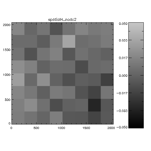
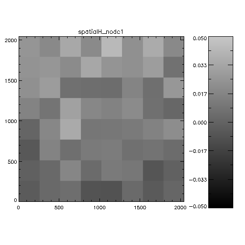
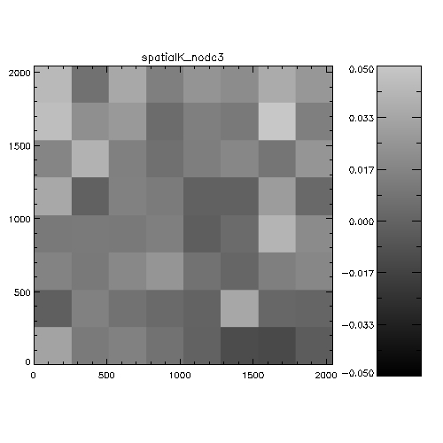
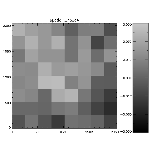
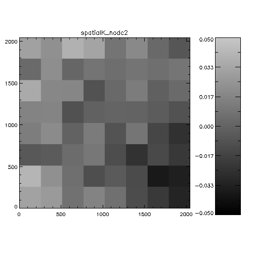
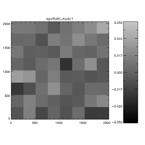
Figure 5: Spatial systematics in WFCAM in the
J-band. For each chip this is the spatially-dependent difference
between 2MASS and WFCAM magnitudes, binned into a 8x8 grid to
improve statistics. The analysis is the stack of a whole night of
observations (20050408). The scale is in magnitudes, and is
WFCAM-2MASS, i.e. white=positive=the objects are fainter in WFCAM
than 2MASS. The colorbars indicate the range of delta magnitudes for
each chip.
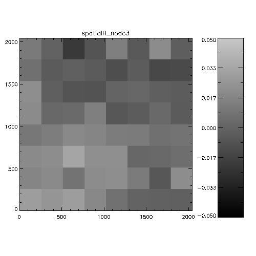
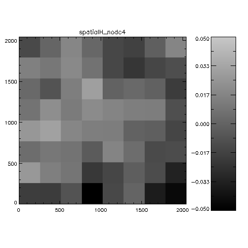
Figure 6: Spatial systematics in WFCAM in the
H-band.
Figure 7: Spatial systematics in WFCAM in the
K-band.
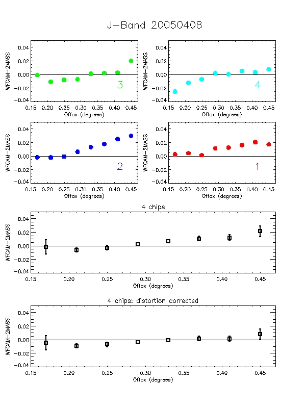
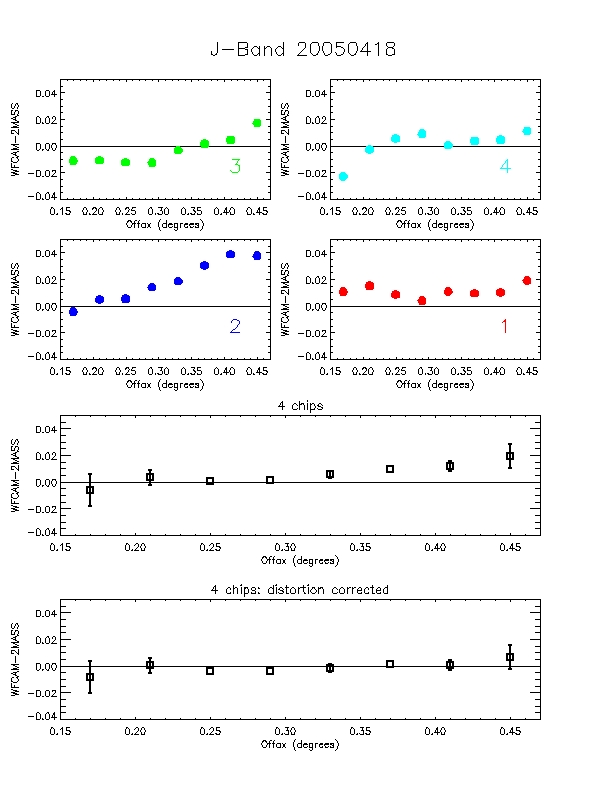
It's hard to see from this whether anything very significant is going
on. An alternative way of investigating the data is to look at WFCAM-2MASS
magnitudes as a function of distance from the rotator centre. the
following 6 plots illustrate this analysis on 2 nights.
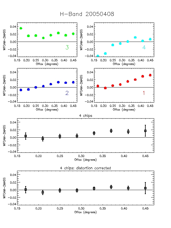
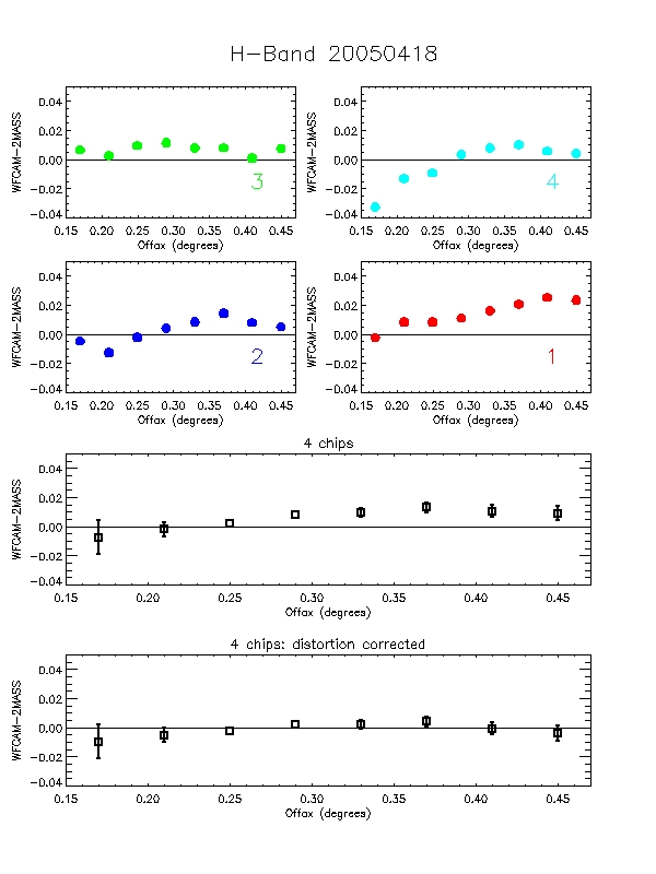
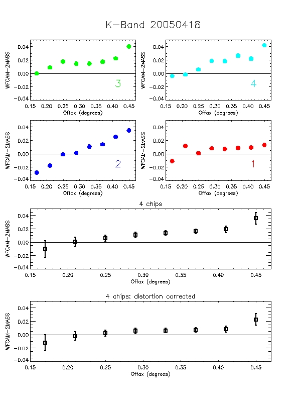
Figure 8: Each of the 6 plots is split into 6 panels. The
top 4 panels (labelled 1-4) show the per-chip variation in WFCAM-2MASS
magnitude as a function of offaxis angle. The bottom two panels are
the median over all 4-chips. The second of these removes the
expected radial distortion contribution to the photometry
(see http://www.ast.cam.ac.uk/~wfcam/docs/reports/astrom/index.html).
At the corners of the field WFCAM has photometry systematics due to
this effect of at most ~1.4% relative to the centre. This is clearly
seen in the above figures. There are also some low level chip-to-chip
variations - but any residual systematics are at about the 1% level
and will need further analysis to really tie down.
3.6.2 From mesostep experiment
We observed a 5x5 grid in two standard fields, offsetting the detector by
1/5 of a detector width each time. We repeated this pattern in each of
ZYJHK filters. I present here the analysis for the J filter in one
field only. Unfortunately this field is a little sparse. It would be
useful to repeat these observations in a very crowded region.
Briefly, I stacked all 25 frames to make a master image, and from this
generated a master catalogue. This is an input list used to drive the
photometry. I then generate a light curve for every object in the
master list. The RMS diagram for these lightcurves is shown below.
 Figure 9: The rms diagram for the mesostepped Field-1 in
the J-band, based on 25 images. Only objects with >=10 data points
are shown in this diagram. Estimated noise contributions are shown
from sky (dash-dot), photon counts (dash) and a systematic fudge
factor of 3 millimags (dot)
Figure 9: The rms diagram for the mesostepped Field-1 in
the J-band, based on 25 images. Only objects with >=10 data points
are shown in this diagram. Estimated noise contributions are shown
from sky (dash-dot), photon counts (dash) and a systematic fudge
factor of 3 millimags (dot)
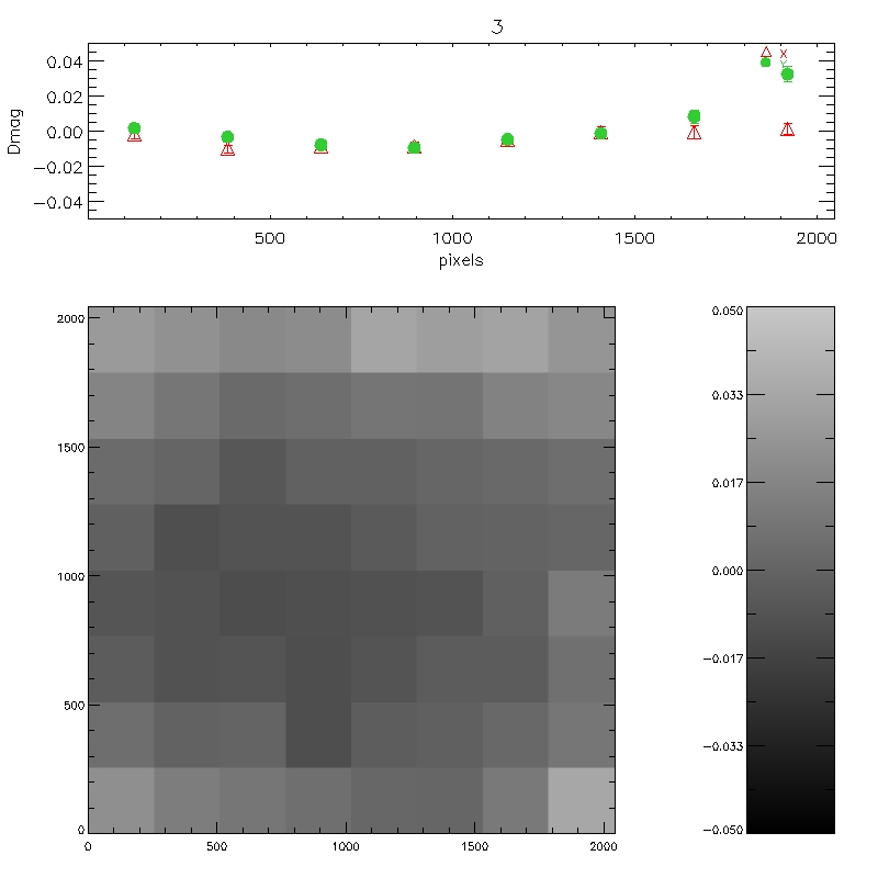
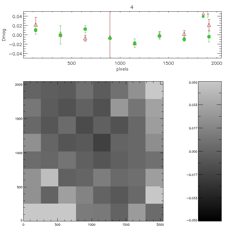
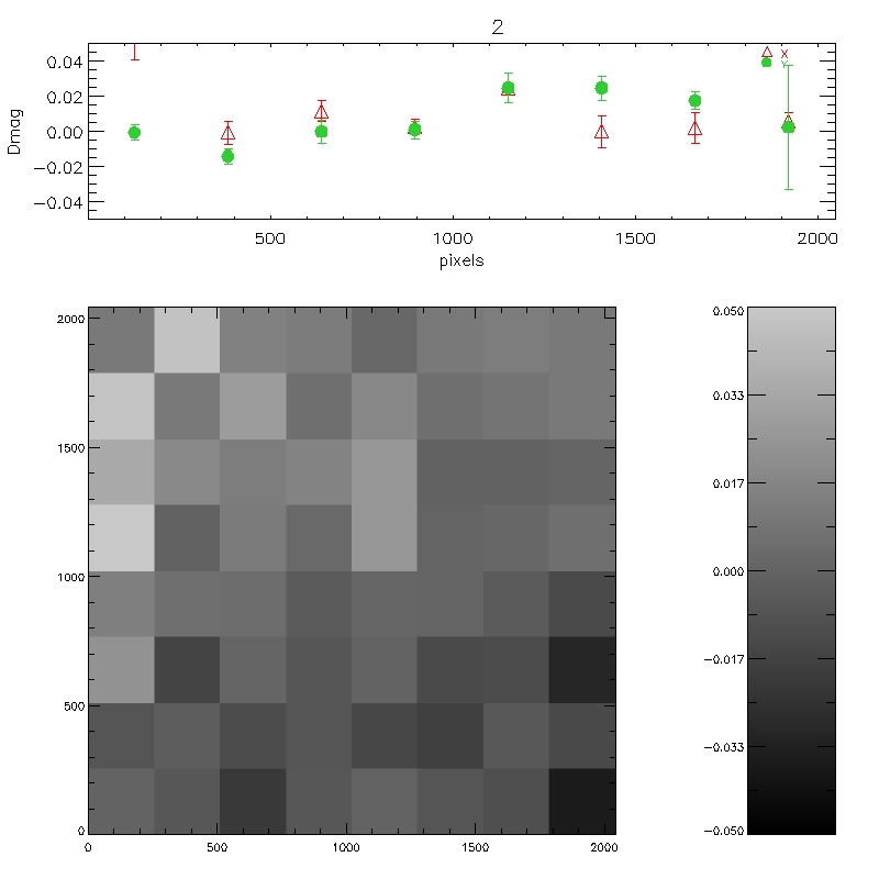
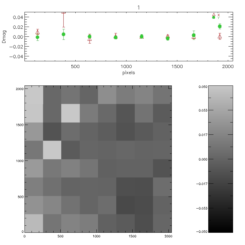
I split each chip into an 8x8 grid. In each cell, I extract the object
lightcurves. For each object (with more than 10 datapooints in the
lightcurve), I then found the median flux of the object, and the
difference between its measurement in this cell, and the median. This
is repeated for all cells and all chips. The results are shown in the
figure below, and again illustrate that there are no systematics at
the >1% level. One could infer this directly from the RMS plot. For
the brightest stars, nothing has an RMS>2%, and most stars with
J<13.0 have RMS values below 1%. I plan to extend this analysis to the
remaining filters, and the second field (which is rather less crowded
than the first).
Figure 10: Mesostep analysis for Field-1, chips 1-4
(clockwise from bottom right) in the J-band. the XY plots are slices
along row 4 and column 4.
4 Pipeline Calibration
4.1 Technique
The pipeline photometric calibration is currently based on 2MASS, via
colour equations to convert to the WFCAM instrumental system. 2MASS
solutions for every catalogued frame are generated and allow
monitoring of effective ZPs at the ~few % level. The 2MASS-WFCAM
colour equations are generated from a large number of catalogued 2MASS
stars observed on the night of UT20050418. The solutions are average
ones, and take no account of, for example, luminosity class. This has
still been done via visual inspection.
ZWFCAM = J2MASS  + 0.95(J-H)2MASS
YWFCAM = J2MASS  + 0.50(J-H)2MASS
JWFCAM = J2MASS - 0.075(J-H)2MASS		(dwarfs: -0.067 giants: -0.003)
HWFCAM = H2MASS + 0.040(J-H)2MASS		(dwarfs: +0.080 giants: +0.065)
KWFCAM = K2MASS - 0.015(J-K)2MASS		(dwarfs: -0.023 giants: +0.032)
The bracketed values are from Steve Warren's analysis of synthetic
colours generated from template spectra (see Hewett et al. 2005) and
Appendix B, which is a copy of an email circulated by Steve Warren.
The CASU derived system zero-points (corrected to unit airmass) for
the main passbands are shown in the next table. Note also that in
deriving these zero-points, all detectors have been gain-corrected to
the average detector system. The CASU pipeline assumes a default
extinction of 0.05 mags/airmass. Thus frame-to-frame variations in
zeropoint include real variations in extinction.
| Zero Point |
Z |
Y |
J |
H |
K |
| WFCAM counts/s |
22.8 |
22.7 |
23.0 |
23.3 |
22.6 |
| WFCAM e-/s |
24.4 |
24.3 |
24.6 |
24.9 |
24.2 |
| UFTI e-/s |
- |
- |
24.5 |
24.7 |
24.2 |
Table 4: WFCAM Zeropoints. The
conversion to electrons assumes an average gain of 5.1.
4.2 Calibration of UKIRT faint standards
For the nights of 20050408 and 20050418 the difference between the
published UFTI photometry for the UKIRT faint standards in the MKO
system has been compared to the pipeline calibrated photometry. The
idea is to see how good a job this first-pass photometric calibration
is doing (Figure 11).
The average offsets (and associated standard deviations) are given in
table 5. The two most significant findings are:
- There is a residual offset in the H-band measurements for the
standards at the 4% level. A closer look at the H_WFCAM to H_2MASS
conversion
(http://www.astro.caltech.edu/~jmc/2mass/v3/transformations/)
shows that this effect was already apparent in the 2MASS colour
equations (see also Carpenter 2001, but note there is no
transformation to MKO, only to the old IRCAM3 system). Since writing
this document, the CASU calibration has altered to include the 4%
offset in H. Figures have not been updated yet to reflect this
change
- The scatter in all filters is rather larger than one might hope
for. At 2-4% it may well represent the limit to how accurately the
WFCAM photometry can be calibrated with 2MASS. Residual spatial
systematics and chip-to-chip variation may also be contributing to
this scatter
 Figure 11: The differences between pipeline calibrated and UFTI
magnitudes for UKIRT faint standards measured on 8th April
2005. J-band in green, H-band in yellow and K-band in red. Horizontal
lines show the mean offset between the CASU and UFTI photometry.
Figure 11: The differences between pipeline calibrated and UFTI
magnitudes for UKIRT faint standards measured on 8th April
2005. J-band in green, H-band in yellow and K-band in red. Horizontal
lines show the mean offset between the CASU and UFTI photometry.
 Figure 12: The differences between pipeline calibrated and UFTI
magnitudes for UKIRT faint standards measured on 18th April
2005. J-band in green, H-band in yellow and K-band in red. Horizontal
lines show the mean offset between the CASU and UFTI photometry.
Figure 12: The differences between pipeline calibrated and UFTI
magnitudes for UKIRT faint standards measured on 18th April
2005. J-band in green, H-band in yellow and K-band in red. Horizontal
lines show the mean offset between the CASU and UFTI photometry.
|
20050408 |
20050418 |
| FILTER |
WFCAM-MKO |
± |
WFCAM-MKO |
± |
| J |
-0.004 |
0.022 |
0.002 |
0.036 |
| H |
0.036 |
0.022 |
0.034 |
0.028 |
| K |
0.016 |
0.020 |
0.006 |
0.023 |
Table 5: UKIRT faint standards calibrated
by the WFCAM pipeline using 2MASS; differences with published
photometry.
Still to do: direct comparison between UFTI and 2MASS systems for
UKIRT faint standards. Is there an inherent offset in the 2MASS
photometry? Now done - see comment above. Add in this effect and
update colour equations
4.3 Calibration of T dwarfs
Figure 13 shows the differences between UFTI and WFCAM photometry for
a series of L and T dwarfs. These stars were observed over a series of
nights. Table 13 summarises the numbers. As with the previous section,
these stars were calibrated via the WFCAM pipeline using 2MASS stars
measured simultaneously.
 Figure 13: The differences between UFTI and WFCAM pipeline
photometry for a series of L and T dwarfs measured as part of SV, as
a function of colour (top) and J magnitude (bottom). J-band is
green, H-band is yellow, K-band is red.
Figure 13: The differences between UFTI and WFCAM pipeline
photometry for a series of L and T dwarfs measured as part of SV, as
a function of colour (top) and J magnitude (bottom). J-band is
green, H-band is yellow, K-band is red.
Principally, there may again be an offset at H, and perhaps at K
(see comments above). However these results are dominated by
the very large scatter in all filters. It's not clear why the scatter
should be as large as 5-8%, given that these stars are not
significantly fainter than the standards. However there are a couple
of factors which may come into play:
- They are observed across a number of nights. It's important to
exclude potentially non-photometric data from this analysis (not yet
done).
- They have spectra that are significantly different from the
standard stars.
- There is a trend for increasing scatter with
increasing magnitude (do we have any estimate for the errors on the
original photometry?)
| FILTER |
WFCAM-MKO |
± |
| J |
0.014 |
0.049 |
| H |
0.075 |
0.078 |
| K |
0.048 |
0.061 |
Table 6: L and T dwarfs calibrated by
the WFCAM pipeline using 2MASS; differences with UFTI
photometry
4.4 Extinction
In this section I will attempt to measure the extinction from the
2MASS data to compare with my derivation from the UKIRT faint
standards.
5 Towards a system of WFCAM secondary standards
This section will describe how the WFCAM secondary standards will be
calibrated from the UKIRT faint standards and collected together to
form a community resource. Ultimately a paper.
6 Summary
6.1 Remaining uncertainties
6.2 Proposed changes to observing strategy?
Appendix A. List of Standards
Appendix B. Synthetic Photometry
Hi Mike

Here are some comments on your WFCAM-2MASS colour equations, based on
an analysis of the synthetic colours. I get mostly pretty good
agreement for dwarfs, but with a few odd effects to note.

Steve

I confined myself to objects of luminosity class III and V in the
BPGS, as well as the additional M dwarfs from Sandy, in Hewett et
al. (2005).

1. Regarding the Z equation you got:

      Z_wfcam  - J2 =  0.95*(J2 - H2)

where J2, H2 are 2MASS. Below I have plotted dwarfs as crosses and
giants as green circles. The red line is your relation, which is
mostly a good fit. But two comments i) the relation goes very badly
wrong for M dwarfs cooler than M3 (become way redder in Z-J2), ii) you
can see from the plot that it seems to turn down very sharply at A0,
so this is something to watch out for. Some of these colours seem
quite odd e.g. A stars with negative Z-Y or Y-J:

    Z-Y     Y-J    class  BPGS no.  name
  -0.069  -0.120   B9V        13  HD189689
  -0.027  -0.094   A0V        14  THETA-VIR
  -0.023  -0.084   B9V        15  NU-CAP
  -0.056  -0.021   A2V        16  HR6169
  -0.022  -0.010   A1V        17  HD190849A
  -0.013  -0.044   A2V        18  69-HER
  -0.009   0.037   A3V        19  HD190849B
  -0.001  -0.050   A0V        20  58-AQL
  -0.029  -0.025   B9V        21  78-HER
  -0.015   0.127   A7V        22  HR6570
   0.028   0.009   A2V        23  HD187754
   0.012   0.083   A5V        24  THETA1-SER
   0.020   0.087   A5V        28  HD190192


2. For the Y band you got

  Y_wfcam  - J2 =  0.50*(J - H)

The analogous plot is below, and you see the same behaviour i.e. cool
M dwarfs very red in Y-J2, and a turndown at zero colour. However in
this plot the scatter looks worse, and the dwarfs and giants may
follow different relations.

I think it would be justified to worry about the usefulness of the
synthetic analysis for the Y band which is probably the band where the
BPGS calibration is worst.  Nevertheless there is a hint that the
relation for dwarfs is somewhat steeper than your value.


  3. J band, you got

    J_wfcam  - J2 =   -0.075*(J2 - H2)

I get somewhat different behaviour for dwarfs and giants

    J_wfcam  - J2 =   0.01-0.067*(J2-H2) dwarfs
    J_wfcam  - J2 =   -0.01-0.003*(J2-H2) giants


4. H band, you got

    H_wfcam  - H2 =  0.075*(J2 - H2)

I get pretty good agreement with that (0.080 for dwarfs and 0.065 for
giants)

5. K band, you got

      K_wfcam  - K2 = - 0.015*(J2 - K2)

The K band is the band where the giants and dwarfs differ the most.

I get
K_wfcam  - K2 = - 0.023*(J2 - K2) (dwarfs)
K_wfcam  - K2 =  -0.01 + 0.032*(J2 - K2)    (giants)

These relations are somewhat non-linear, and so the colour term
depends on the colour range selected.