Interpolation tests
Interpolation tests
Document number: VDF-TRE-IOA-00016-0002 Version 1
Dafydd Wyn Evans & Mike Irwin, IoA
13 November 2003
1 Introduction
The purpose of this document is to look into the effects of interpolation on
pixel data.
There are a number of procedures in the processing of WFCAM data which will
require the interpolation of pixel data. These are mainly to do with
procedures that need matched pixel grids. These include the stacking of
data, the creation of contiguous tiled mosaics, PSF fitting and difference
imaging.
As an example, when pixel data is stacked, it is usually the case that the
pixels from the
different images do not match up perfectly. This could be due to a pointing
error, in the case of direct stacking, or image distortion ([Irwin 2003])
at the edge of a frame, in the case of overlaps. In these situations the
data must be resampled so that it matches the desired pixel grid and this
is done by interpolating the data.
In an ideal case sinc(x) interpolation is perfect for band-limited data
(Shannon's sampling theorem). However,
in practice the need for infinite support in the spatial
domain makes sinc(x) interpolation impractical.
Also the presence of negative weights
cause the interpolated image to suffer from ringing (Gibb's phenomenon)
since real data is not
band-limited. Because of its theoretical attractiveness,
sinc(x) interpolation gives rise to a whole variety of
similar methods, not just windowed sinc(x).
2 SWarp
For this investigation the interpolation was carried out using the
SWarp
programme written by Emmanuel Bertin. This programme resamples and co-adds
images using any WCS defined astrometric projection. For this work, it was
only the resampling/interpolation part of the programme that was used.
The interpolation methods tested out were:
- NEAREST
- Nearest neighbour interpolation simply uses the value from
the nearest pixel. In terms of a convolution kernel this is a square top hat
function, with width 1 pixel.
- BILINEAR
- A pyramidal response function with a FWHM of 1 pixel. This
results in a bilinear interpolation.
- LANCZOS2
- Lanczos-2 4-tap filter ie. sinc(πx)sinc(πx/2) for |x| < 2
- LANCZOS3
- Lanczos-3 6-tap filter ie. sinc(πx)sinc(πx/3) for |x| < 3
- LANCZOS4
- Lanczos-4 8-tap filter ie. sinc(πx)sinc(πx/4) for |x| < 4
The Lanczos methods belong to the general class of windowed sinc(x)
interpolation methods.
There are other common interpolation schemes that may be
appropriate for certain applications that are not available in SWarp
and that need considering eg. Hann/Hamming, hyperbolic tangent, bi-cubic
spline.
Bertin kindly provided a pre-release version (2.0b8) of the latest software.
3 How the interpolation is carried out
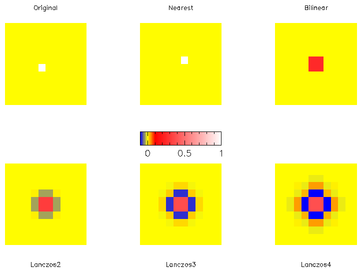
In order to give a better feel on how the interpolation is carried out for
the different resampling methods an image was created with the background
set to 0.0 and one pixel at 1.0 (equivalent to a delta function). A resampling
was then carried out with a simple shift of 0.5 both in x and y for the
entire frame. The resulting images (shown in
Figure 1) are effectively the weights that are applied to
generate a
resampled image for this transformation (a simple shift in this case).
Figure 1: Examples of a resampled image (a delta function) using different
interpolation methods. The transformation from the original is a simple
shift of 0.5 both in x and y for the entire frame.
The numerical values for this shift are given in Appendix A.
Using these values the reduction in the pixel noise variance can be
calculated from
where Mij are the pixel interpolation weights with ∑ij Mij=1
to conserve flux. In the worst case, a bilinear interpolation for a shift of
0.5 pixels in both coordinates, a reduction by a factor of 4 is seen in the
variance.
4 The simulations carried out
The source data used in these tests were the same simulations as generated
in [Evans 2003]. The resampling was carried out on the
interleaved (2×2) data.
Three different sets of simulations were tested, each with different
seeing conditions:
-
All four elements of the interleaved images were generated with the
same seeing (0.6").
-
Realistic seeing conditions - seeing is within 0.1" of
the median.
Each of the four elements had a randomly determined seeing taken from a
Gaussian
distribution with a mean of 0.6" and a sigma of 0.05".
-
Bad seeing conditions - seeing suddenly increases by 0.5". The
seeing is determined as in b, but for the fourth element the seeing is
increased by 0.5".
Five different transformations were carried out for each case, including for
each interpolation method (see Table 1). All of them were simple
shift transformations
ranging from 0.05 to 0.5 pixels. No shifts above 0.5 were tested since the
interpolation methods are all symmetric.
Different shifts were applied in x and y in order to reduce the number
of frames produced.
| Transformation | Shift/pixels |
| x | y |
| 1 | 0.05 | 0.10 |
| 2 | 0.15 | 0.20 |
| 3 | 0.25 | 0.30 |
| 4 | 0.35 | 0.40 |
| 5 | 0.45 | 0.50 |
Table 1: The five different transformations applied to all images.
5 Analysis
The analysis of the resampled data consisted of reducing it using the programme
imcore_conf, the standard source detection and parameterization
programme used in CASU pipelines. Further information about how
imcore_conf works can be found in [Irwin 1996]. The output from
these reductions used in these comparisons were x, y and flux, where
the flux is measured with respect to a
locally smooth sky estimate using an aperture of width of twice the FWHM.
These were then compared with the true
values used to generate the simulations.
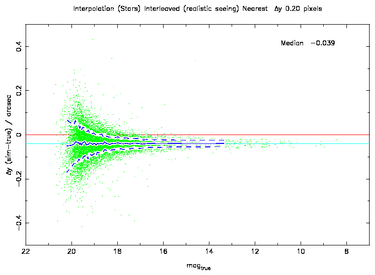
Not only does this show up any
systematic effects, but also the widths of these
distributions as a function of magnitude (see
Figure 2) gives a reasonable estimate for the errors in
these parameters.
Figure 2: The residuals in position as a function of magnitude. The solid blue
line shows the median of the distribution and the dashed blue line indicates
the width (equivalent to a Gaussian sigma). The offset seen agrees with the
transformation offset (scale 0.2"/pixel), as expected for nearest
neighbour interpolation.
The following summaries apply to all 3 seeing conditions simulated since no
significant difference was seen between them.
5.1 Astrometric offset
The most obvious effect is that NEAREST will display an offset equal to the
size of the relevant shift used in the transformation ie. between 0.05 and
0.5 pixels.
BILINEAR showed no offsets, while LANCZOS2 had small offsets of up to 0.025
pixels for a 0.5 pixel shift. LANCZOS3 and LANCZOS4 showed similar behaviour
to LANCZOS2, but were smaller.
5.2 Astrometric errors
For the NEAREST errors no difference is seen.
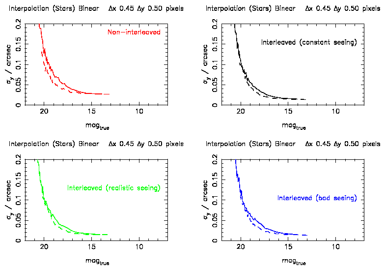
For BILINEAR, starting at a shift of 0.15 pixel, there is an increase in the
astrometric error at about 18th magnitude. The errors at the bright and
faint end stay the same. This increase in error increases with pixel shift.
For a shift of 0.5 pixel the increase is from 0.025" to 0.035" at 18th
magnitude (see Figure 3).
Figure 3: Astrometric errors as a function of magnitude for bilinear
interpolation with a 0.5 pixel shift. The results
from the different seeing conditions are in different colours. The dashed
line is the same analysis for the non-resampled data.
LANCZOS2 shows similar behaviour to BILINEAR, but the increase starts at
shifts of about 0.25 pixel. Similarly LANCZOS3 starts showing the increase
at 0.35 pixel. LANCZOS4 shows no increase in astrometric error whatever the
transformation shift.
5.3 Photometric offset
At the millimagnitude level, no photometric offsets are seen, whatever the
interpolation method or the transformation shift. This is expected with
the flux measure used since the definition of the interpolation weights
implies conservation of flux for regular sampling.
5.4 Photometric errors
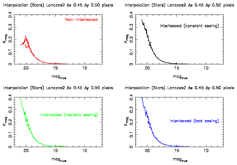
Very little change is also seen in the photometric errors due to interpolation.
Possibly for LANCZOS2 the errors are slightly larger at the faint end for
the largest shifts (see Figure 4).
Figure 4: Photometric errors as a function of magnitude for Lanczos2
interpolation with a 0.5 pixel shift. The results
from the different seeing conditions are in different colours. The dashed
line is the same analysis for the non-resampled data.
5.5 Noise properties
The main change that occurs for resampled data is that
the noise properties of the image changes. This is because for each method
(except NEAREST) some form of local averaging (convolution) is carried out.
This is not unexpected since each method involves an implicit convolution.
This operation will be reflected in the noise
covariance matrix. Examples of these are given in Appendix B for
a shift of 0.5 pixels in both coordinates.
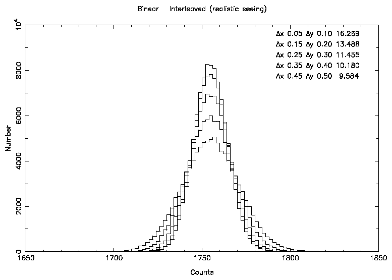
Figure 5: This diagram shows the change in noise properties as the
transformation shift is increased for bilinear interpolation.
Using a robust estimator for determining the noise level for each frame, it
can be shown that the noise level decreases with increasing pixel shift up to
0.5 pixel for each interpolation method.
The exception is NEAREST, for which no changes in the noise properties occurs.
BILINEAR displays the most extreme case with the noise reducing by a factor
of 2. This can be seen in Figure 5. Even with small shifts
the noise level is reduced from 18.9 to 16.3 counts. These reductions agree
with the predictions from the formula given in Section 3.
Visually inspecting the images also reveals a clumpy nature to the background.
This is quantified by the noise covariance matrices (see AppendixB).
LANCZOS2 shows a smaller reduction in noise level and similarly for LANCZOS3
and LANCZOS4. For LANCZOS4 the reduction in noise for the worst case is from
18.9 to 15.7 counts.
Although the pixel noise variance has been reduced, the non-zero terms of
the rest of the noise covariance matrix quantify the redistribution of the
spatial noise characteristics.
These changes in the noise properties will have interesting consequences for
any transformation other than simple shifts since the noise properties will
then vary across the field.
6 A more general transformation
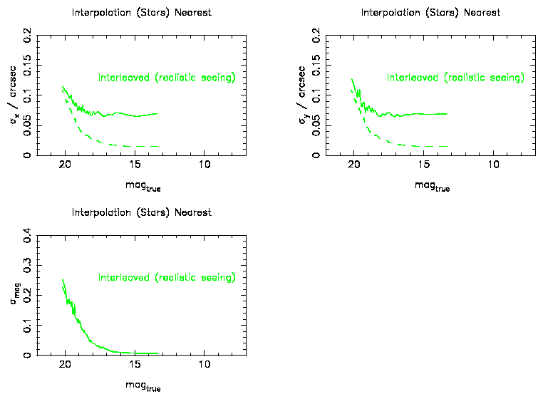
Figure 6: Astrometric and photometric errors as a function of magnitude
for nearest neighbour
interpolation for a transformation consisting of a small rotation and change
in scale. The dashed line is the same analysis for the non-resampled data.
In order to test out a more realistic transformation, resampling tests were
carried out for a combined rotation and scale change. The rotation was such
that it would amount to a 5 pixel shift at the frame edge and
the scale factor was also chosen so that it would amount to similar shift at
the edge. This effectively samples all possible sub-pixel shifts.
The astrometric and photometric error analysis shows no significant
differences from the sort of behaviour seen in the previous section except
for NEAREST. In this case
there is effectively an additional error of 0.07" (about a third of a pixel)
caused by the resampling (see Figure 6). This is due to the
systematic errors of between 0.0 and 0.5 pixel occurring across the field.
This would rule out nearest neighbour interpolation for consideration for
WFCAM where precise astrometry is needed.
However, it may be possible to construct some form of correction map for
the derived parameters from a resampled image.
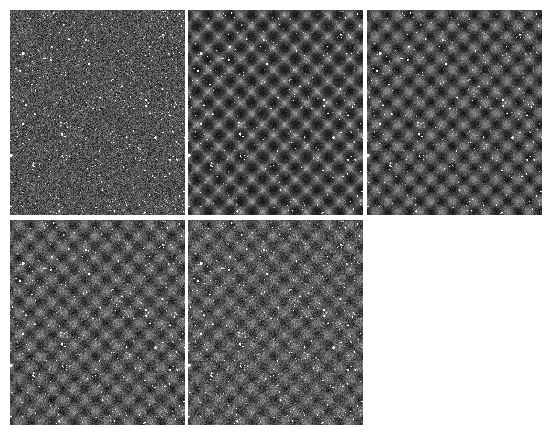
Figure 7: This diagram shows the change in noise levels across a frame for a
transformation consisting of a small rotation and change
in scale. The order of the plots is (top row) NEAREST, BILINEAR and LANCZOS2
(bottom row) LANCZOS3 and LANCZOS4. The greyscale is the same for each plot.
If you measure the noise level as a function of position you see a grid
pattern for all methods except NEAREST (see Figure 7). This is
simply a consequence of the local shifts (modulo a pixel) varying across the
field. In some areas the pixel grid will match that of the original frame
and thus the interpolation will be perfect since no averaging across many
pixels is required. The change in noise levels between the troughs and
ridges is the same as that seen in Section 5.5.
7 Conclusions
The choice of the best interpolation method will depend on what is going to
be done with the data.
- If you want noise properties the same as in the original data, then you
should use NEAREST (see Figure 7).
- If you don't want ringing, then you should avoid Lanczos or other sinc
methods. Methods that don't display ringing are bilinear or Hann/Hamming
interpolation.
- If you want to do precise astrometry, then you should avoid NEAREST (see
Figure 6) and use LANCZOS3 or LANCZOS4.
Future work:
- Effect of interpolation on profile fitting.
- Investigate other common interpolation schemes eg. Hann/Hamming,
hyperbolic tangent, bi-cubic spline.
A postscript version of this report can be found at
http://www.ast.cam.ac.uk/~wfcam/docs/reports/interpol/interpol.ps.
References
- [Evans 2003]
-
Evans D.W., 2003. Internal report
http://www.ast.cam.ac.uk/~wfcam/docs/reports/interleaving/
`Interleaving tests'
- [Irwin 1996]
-
Irwin M.J.,
1996, Instrumentation for Large Telescopes,
VII Canary Islands Winter School, eds. J.M.Rodríguez
Espinosa, A.Herrero, F.Sánchez, p. 35.
`Detectors and Data Analysis Techniques for Wide Field Optical
Imaging'
also available from
http://www.ast.cam.ac.uk/~mike/processing.ps.gz
- [Irwin 2003]
-
Irwin M.J., 2003. Internal report
http://www.ast.cam.ac.uk/~wfcam/docs/reports/astrom/
`Astrometric Distortion for WFCAM and VISTA'
A Weighting values for a (0.5,0.5) shift
This appendix contains the weighting values for a (0.5,0.5) shift for each
interpolation method. An image consisting of a single pixel (see
Table 2) is transformed and resampled to generate
Tables 3 to 7.
| 0.0000 | 0.0000 | 0.0000 | 0.0000 | 0.0000 | 0.0000 | 0.0000 | 0.0000 |
| 0.0000 | 0.0000 | 0.0000 | 0.0000 | 0.0000 | 0.0000 | 0.0000 | 0.0000 |
| 0.0000 | 0.0000 | 0.0000 | 0.0000 | 0.0000 | 0.0000 | 0.0000 | 0.0000 |
| 0.0000 | 0.0000 | 0.0000 | 1.0000 | 0.0000 | 0.0000 | 0.0000 | 0.0000 |
| 0.0000 | 0.0000 | 0.0000 | 0.0000 | 0.0000 | 0.0000 | 0.0000 | 0.0000 |
| 0.0000 | 0.0000 | 0.0000 | 0.0000 | 0.0000 | 0.0000 | 0.0000 | 0.0000 |
| 0.0000 | 0.0000 | 0.0000 | 0.0000 | 0.0000 | 0.0000 | 0.0000 | 0.0000 |
| 0.0000 | 0.0000 | 0.0000 | 0.0000 | 0.0000 | 0.0000 | 0.0000 | 0.0000 |
Table 2: The original image/matrix before resampling and generating
Tables 3 to 7.
| 0.0000 | 0.0000 | 0.0000 | 0.0000 | 0.0000 | 0.0000 | 0.0000 | 0.0000 |
| 0.0000 | 0.0000 | 0.0000 | 0.0000 | 0.0000 | 0.0000 | 0.0000 | 0.0000 |
| 0.0000 | 0.0000 | 0.0000 | 0.0000 | 0.0000 | 0.0000 | 0.0000 | 0.0000 |
| 0.0000 | 0.0000 | 0.0000 | 0.0000 | 0.0000 | 0.0000 | 0.0000 | 0.0000 |
| 0.0000 | 0.0000 | 0.0000 | 0.0000 | 1.0000 | 0.0000 | 0.0000 | 0.0000 |
| 0.0000 | 0.0000 | 0.0000 | 0.0000 | 0.0000 | 0.0000 | 0.0000 | 0.0000 |
| 0.0000 | 0.0000 | 0.0000 | 0.0000 | 0.0000 | 0.0000 | 0.0000 | 0.0000 |
| 0.0000 | 0.0000 | 0.0000 | 0.0000 | 0.0000 | 0.0000 | 0.0000 | 0.0000 |
Table 3: Pixel interpolation weights for NEAREST for a (0.5,0.5) shift.
| 0.0000 | 0.0000 | 0.0000 | 0.0000 | 0.0000 | 0.0000 | 0.0000 | 0.0000 |
| 0.0000 | 0.0000 | 0.0000 | 0.0000 | 0.0000 | 0.0000 | 0.0000 | 0.0000 |
| 0.0000 | 0.0000 | 0.0000 | 0.0000 | 0.0000 | 0.0000 | 0.0000 | 0.0000 |
| 0.0000 | 0.0000 | 0.0000 | 0.2500 | 0.2500 | 0.0000 | 0.0000 | 0.0000 |
| 0.0000 | 0.0000 | 0.0000 | 0.2500 | 0.2500 | 0.0000 | 0.0000 | 0.0000 |
| 0.0000 | 0.0000 | 0.0000 | 0.0000 | 0.0000 | 0.0000 | 0.0000 | 0.0000 |
| 0.0000 | 0.0000 | 0.0000 | 0.0000 | 0.0000 | 0.0000 | 0.0000 | 0.0000 |
| 0.0000 | 0.0000 | 0.0000 | 0.0000 | 0.0000 | 0.0000 | 0.0000 | 0.0000 |
Table 4: Pixel interpolation weights for BILINEAR for a (0.5,0.5) shift.
| 0.0000 | 0.0000 | 0.0000 | 0.0000 | 0.0000 | 0.0000 | 0.0000 | 0.0000 |
| 0.0000 | 0.0000 | 0.0000 | 0.0000 | 0.0000 | 0.0000 | 0.0000 | 0.0000 |
| 0.0000 | 0.0000 | 0.0039 | -0.0352 | -0.0352 | 0.0039 | 0.0000 | 0.0000 |
| 0.0000 | 0.0000 | -0.0352 | 0.3164 | 0.3164 | -0.0352 | 0.0000 | 0.0000 |
| 0.0000 | 0.0000 | -0.0352 | 0.3164 | 0.3164 | -0.0352 | 0.0000 | 0.0000 |
| 0.0000 | 0.0000 | 0.0039 | -0.0352 | -0.0352 | 0.0039 | 0.0000 | 0.0000 |
| 0.0000 | 0.0000 | 0.0000 | 0.0000 | 0.0000 | 0.0000 | 0.0000 | 0.0000 |
| 0.0000 | 0.0000 | 0.0000 | 0.0000 | 0.0000 | 0.0000 | 0.0000 | 0.0000 |
Table 5: Pixel interpolation weights for LANCZOS2 for a (0.5,0.5) shift.
| 0.0000 | 0.0000 | 0.0000 | 0.0000 | 0.0000 | 0.0000 | 0.0000 | 0.0000 |
| 0.0000 | 0.0006 | -0.0033 | 0.0150 | 0.0150 | -0.0033 | 0.0006 | 0.0000 |
| 0.0000 | -0.0033 | 0.0185 | -0.0831 | -0.0831 | 0.0185 | -0.0033 | 0.0000 |
| 0.0000 | 0.0150 | -0.0831 | 0.3738 | 0.3738 | -0.0831 | 0.0150 | 0.0000 |
| 0.0000 | 0.0150 | -0.0831 | 0.3738 | 0.3738 | -0.0831 | 0.0150 | 0.0000 |
| 0.0000 | -0.0033 | 0.0185 | -0.0831 | -0.0831 | 0.0185 | -0.0033 | 0.0000 |
| 0.0000 | 0.0006 | -0.0033 | 0.0150 | 0.0150 | -0.0033 | 0.0006 | 0.0000 |
| 0.0000 | 0.0000 | 0.0000 | 0.0000 | 0.0000 | 0.0000 | 0.0000 | 0.0000 |
Table 6: Pixel interpolation weights for LANCZOS3 for a (0.5,0.5) shift.
| 0.0002 | -0.0008 | 0.0021 | -0.0078 | -0.0078 | 0.0021 | -0.0008 | 0.0002 |
| -0.0008 | 0.0036 | -0.0099 | 0.0370 | 0.0370 | -0.0099 | 0.0036 | -0.0008 |
| 0.0021 | -0.0099 | 0.0276 | -0.1027 | -0.1027 | 0.0276 | -0.0099 | 0.0021 |
| -0.0078 | 0.0370 | -0.1027 | 0.3830 | 0.3830 | -0.1027 | 0.0370 | -0.0078 |
| -0.0078 | 0.0370 | -0.1027 | 0.3830 | 0.3830 | -0.1027 | 0.0370 | -0.0078 |
| 0.0021 | -0.0099 | 0.0276 | -0.1027 | -0.1027 | 0.0276 | -0.0099 | 0.0021 |
| -0.0008 | 0.0036 | -0.0099 | 0.0370 | 0.0370 | -0.0099 | 0.0036 | -0.0008 |
| 0.0002 | -0.0008 | 0.0021 | -0.0078 | -0.0078 | 0.0021 | -0.0008 | 0.0002 |
Table 7: Pixel interpolation weights for LANCZOS4 for a (0.5,0.5) shift.
B Noise covariance matrices
Tables 8 to 12 are the noise covariance matrices for
a (0.5,0.5) shift using different interpolation methods. The data transformed
was a frame with no images in it with a bias of 100 and a noise level of 10.
This frame was transformed and interpolated by SWarp and then the noise
covariance matrix calculated.
| 0.000 | 0.000 | 0.000 | 0.000 | 0.000 | 0.000 | 0.000 | 0.000 | 0.000 |
| 0.000 | 0.000 | 0.000 | 0.000 | 0.000 | 0.000 | 0.000 | 0.000 | 0.000 |
| 0.000 | 0.001 | 0.000 | 0.000 | 0.000 | 0.000 | 0.000 | 0.000 | 0.000 |
| 0.000 | 0.000 | 0.000 | 0.000 | 0.000 | 0.000 | 0.000 | 0.000 | 0.000 |
| 0.000 | 0.000 | 0.000 | 0.000 | 1.000 | 0.000 | 0.000 | 0.000 | 0.000 |
| 0.000 | 0.000 | 0.000 | 0.000 | 0.000 | 0.000 | 0.000 | 0.000 | 0.000 |
| 0.000 | 0.000 | 0.000 | 0.000 | 0.000 | 0.000 | 0.000 | 0.001 | 0.000 |
| 0.000 | 0.000 | 0.000 | 0.000 | 0.000 | 0.000 | 0.000 | 0.000 | 0.000 |
| 0.000 | 0.000 | 0.000 | 0.000 | 0.000 | 0.000 | 0.000 | 0.000 | 0.000 |
Table 8: The noise covariance matrix for NEAREST with a (0.5,0.5)
shift.
| 0.001 | 0.000 | 0.000 | 0.000 | 0.000 | 0.000 | 0.000 | 0.000 | 0.000 |
| 0.000 | 0.000 | 0.000 | 0.000 | 0.000 | 0.000 | 0.000 | 0.001 | 0.000 |
| 0.000 | 0.000 | 0.000 | 0.000 | 0.000 | 0.000 | 0.000 | 0.000 | 0.000 |
| 0.000 | 0.000 | 0.000 | 0.247 | 0.494 | 0.247 | 0.000 | 0.000 | 0.000 |
| 0.000 | 0.000 | 0.000 | 0.494 | 1.000 | 0.494 | 0.000 | 0.000 | 0.000 |
| 0.000 | 0.000 | 0.000 | 0.247 | 0.494 | 0.247 | 0.000 | 0.000 | 0.000 |
| 0.000 | 0.000 | 0.000 | 0.000 | 0.000 | 0.000 | 0.000 | 0.000 | 0.000 |
| 0.000 | 0.001 | 0.000 | 0.000 | 0.000 | 0.000 | 0.000 | 0.000 | 0.000 |
| 0.000 | 0.001 | 0.000 | 0.000 | 0.000 | 0.000 | 0.000 | 0.000 | 0.000 |
Table 9: The noise covariance matrix for BILINEAR with a (0.5,0.5)
shift.
| 0.001 | 0.000 | 0.000 | 0.000 | 0.000 | 0.000 | 0.000 | 0.000 | 0.000 |
| 0.000 | 0.000 | -0.001 | 0.003 | 0.006 | 0.002 | -0.001 | 0.001 | 0.000 |
| 0.000 | 0.000 | 0.012 | -0.042 | -0.108 | -0.042 | 0.012 | -0.001 | 0.000 |
| 0.000 | 0.003 | -0.042 | 0.146 | 0.379 | 0.146 | -0.041 | 0.002 | 0.000 |
| 0.000 | 0.006 | -0.108 | 0.379 | 1.000 | 0.379 | -0.108 | 0.006 | 0.000 |
| 0.000 | 0.002 | -0.041 | 0.146 | 0.379 | 0.146 | -0.042 | 0.003 | 0.000 |
| 0.000 | 0.000 | 0.012 | -0.042 | -0.108 | -0.041 | 0.012 | 0.000 | 0.000 |
| 0.000 | 0.001 | 0.000 | 0.002 | 0.006 | 0.003 | -0.001 | 0.000 | 0.000 |
| 0.000 | 0.001 | 0.000 | 0.000 | 0.000 | 0.000 | 0.000 | 0.000 | 0.001 |
Table 10: The noise covariance matrix for LANCZOS2 with a (0.5,0.5)
shift.
| 0.001 | -0.001 | 0.002 | -0.002 | -0.009 | -0.003 | 0.002 | 0.000 | 0.000 |
| 0.000 | 0.004 | -0.011 | 0.016 | 0.061 | 0.015 | -0.010 | 0.004 | 0.000 |
| 0.002 | -0.010 | 0.029 | -0.044 | -0.171 | -0.044 | 0.030 | -0.010 | 0.002 |
| -0.002 | 0.016 | -0.044 | 0.065 | 0.253 | 0.065 | -0.044 | 0.016 | -0.002 |
| -0.008 | 0.061 | -0.171 | 0.253 | 1.000 | 0.252 | -0.171 | 0.061 | -0.008 |
| -0.002 | 0.016 | -0.043 | 0.065 | 0.253 | 0.065 | -0.044 | 0.016 | -0.002 |
| 0.002 | -0.010 | 0.030 | -0.044 | -0.170 | -0.044 | 0.029 | -0.010 | 0.002 |
| 0.000 | 0.005 | -0.010 | 0.015 | 0.061 | 0.016 | -0.011 | 0.004 | 0.000 |
| 0.001 | 0.000 | 0.002 | -0.002 | -0.008 | -0.002 | 0.002 | -0.001 | 0.001 |
Table 11: The noise covariance matrix for LANCZOS3 with a (0.5,0.5)
shift.
| 0.002 | -0.004 | 0.006 | -0.007 | -0.005 | 0.027 | 0.041 | 0.031 | 0.037 |
| -0.004 | 0.010 | -0.015 | 0.018 | 0.130 | 0.052 | 0.020 | 0.045 | 0.031 |
| 0.006 | -0.014 | 0.022 | -0.027 | -0.106 | 0.008 | 0.056 | 0.020 | 0.041 |
| -0.007 | 0.018 | -0.026 | 0.033 | 0.208 | 0.067 | 0.008 | 0.053 | 0.028 |
| -0.004 | 0.130 | -0.106 | 0.208 | 1.000 | 0.242 | -0.072 | 0.164 | 0.030 |
| 0.028 | 0.053 | 0.008 | 0.067 | 0.242 | 0.102 | 0.043 | 0.087 | 0.062 |
| 0.041 | 0.020 | 0.056 | 0.008 | -0.072 | 0.043 | 0.091 | 0.055 | 0.075 |
| 0.031 | 0.045 | 0.020 | 0.052 | 0.164 | 0.087 | 0.054 | 0.079 | 0.065 |
| 0.037 | 0.031 | 0.041 | 0.027 | 0.030 | 0.062 | 0.075 | 0.065 | 0.071 |
Table 12: The noise covariance matrix for LANCZOS4 with a (0.5,0.5)
shift.
LANCZOS4 possibly has a bug in it since it
is not symmetric. I have emailed Bertin
File translated from
TEX
by
TTH,
version 3.30.
On 14 Nov 2003, 17:21.