All the data has been read onto RAID disks and converted, first to single extension FITS using an equivalent of the summit ORAC-DR conversion script, and then finally to MEF format - ie. one FITS container file for all 4 detectors.
The data taking system stablilised by the first week of November and most of the useful commissioning data results from then onwards.
The on-sky layout of the detectors is shown below. The green marker is the "bottom-left" corner on a default display ie. the pixel 1,1. The x (fastest varying) and y axes are shown for each detector. Note that all detector images output from the DAS are inverted with respect to astronomical sky and that each detector image is rotated through 90 degrees with respect to the next detector in the sequence.
More detailed measurements of the detector location with respect to the optical axis and each other are presented in a later section.
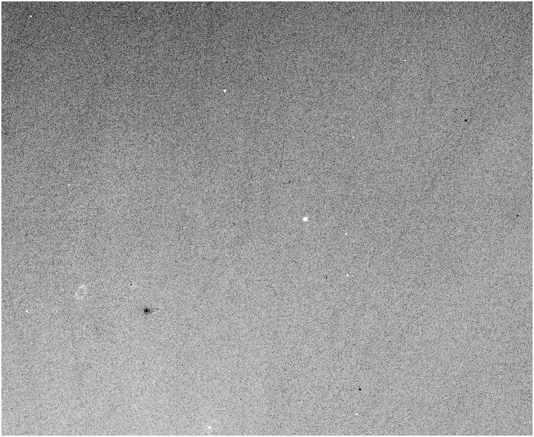
The analysis was based on quick-look processing of (essentially) self-calibrating 9-point jitter sequences. An example individual raw K-band frame for detector #2 covering about 1/2 the area is shown below.
The first processing step is to subtract stacked dark frames of the same exposure time as the science frames. Then for each set of 9 exposures a flatfield frame was made by combining the dark-corrected individual frames in each jitter sequence. An example of this for the same detector and region used in the previous example is shown below.
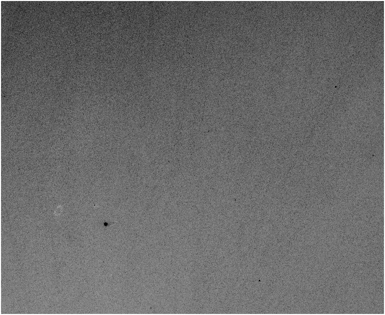
Applying this flatfield frame to this region gives the result frame shown below. Given the absence of measurable fringing ( << 1% in Z,Y,J,H,K measured using twilight flats to flatfield combined dark sky frames) in any of the passbands studied so far this is adequate for analysis of most objects in the frames.
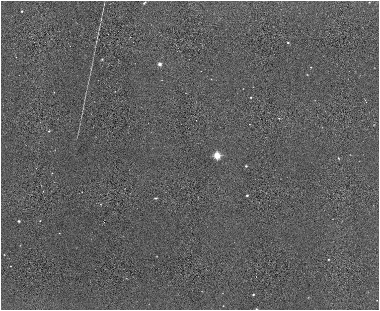
Object catalogues are then generated for all frames, an astrometric solution is made using the catalogues and used to update the WCS in the image headers. The final image processing step is to stack the 9 jitter frames for each sequence and an example of the result of this is shown next.
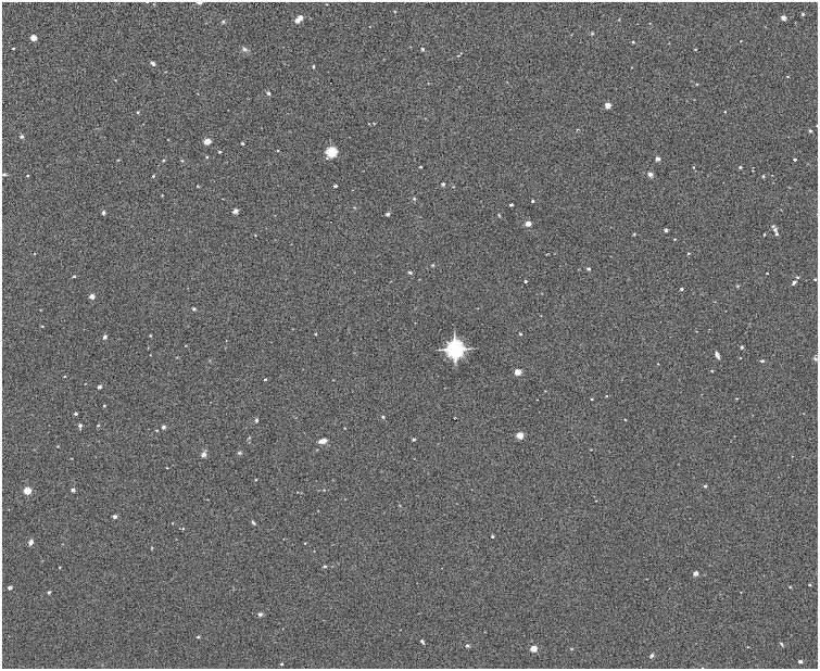
Note the vanished "trail" from the individual image, the greatly increased depth, and the very slight halo around the bright star in the centre - a consequence of the self-flat process. This latter effect is at the level of around ~2 counts cf. to the sky level of ~5500 counts.
more on noise chars .............
In doing the processing a first order on-sky estimate of the gain (e-/ADU) of the detectors was made by subtracting two consecutive raw K-band images and analysing the noise in the difference image using a robust estimator (since obviously bits of objects are also present - the estimator also allows for any residual differential smooth changes in background). Allowing for the dark frame variance (the robust measured noise levels in the difference between 2 single exposure darks are: 9.6, 8.0, 8.1, 8.1) gives the following results:-
Sky level   = 7027.8
Noise level =   32.0 var{} = noise**2*3/2 = 1536 - 46 = 1490/exposure gain 4.7
Sky level   = 6755.8
Noise level =   31.3       etc.                         1438               4.7
Sky level   = 6318.9
Noise level =   28.0                                    1143               5.5
Sky level   = 6270.1
Noise level =   28.9                                    1220               5.1
NB. Each frame used is a coaverage of 3 exposures.
The main assumptions in the gain calculation are namely: that the dominating noise source after allowing for dark noise is photon noise and that for the bluer passbands the reset-anomaly was removed reasonably well using the darks. The expected gain was of order 4, but note that this needs doing more thoroughly using sequences of dome flats after the non-linearity has been characterised.
[NB. At this stage we have not yet characterised the WFCAM non-linearity so we are also assuming that this is small ie. a few % or less at these levels. This assumption obviously also applies to the photometric sensitvity measurements. Differences in non-linearity between the detectors will also affect the measured relative sensitivities.]
For the Lockman Hole dataset the sensitivity in each passband (assuming uniform illumination on average) is simply derived by comparing robust estimates of the average dark-corrected background level in each detector (assuming good average reset-anomaly removal) and then applying the gains above. This was further refined using a series of dawn twilight sky flats taken over several nights. The relative sensivity in counts (ADU) and detected electrons (e-) is given below:
J-band                       #1     #2     #3     #4
Sensitivity relative to #1  1.00   0.92   0.94   0.79    (ADU)
                            1.00   0.92   1.10   0.86    (e-)
H-band
Sensitivity relative to #1  1.00   0.92   0.89   0.80    (ADU)
                            1.00   0.92   1.04   0.87    (e-)
K-band
Sensitivity relative to #1  1.00   0.94   0.86   0.83    (ADU)
                            1.00   0.94   1.02   0.91    (e-)
Y-band
Sensitivity relative to #1  1.00   0.92   0.97   0.77    (ADU)
                            1.00   0.92   1.13   0.84    (e-)
Z-band
Sensitivity relative to #1  1.00   0.93   0.97   0.75    (ADU)
                            1.00   0.93   1.13   0.82    (e-)
from which you can work out the relative ZPs using the table of photometric
ZPs on the average detector system toward the end of this document.
See later table for a list of average photometric zero-points.
Note that the noise properties and full well consistent with gains.
For general information on the effects of the field distortion see the WFCAM and VISTA astrometry report .
In the following tests we have used the 2MASS PSC as the basis for all the astrometry. The results are very promising and we intend to use 2MASS for all astometric calibration for WFCAM. Note that 2MASS astrometry is based on Tycho 2 and is in the International Celestial Reference System (ICRS). This does not require an Equinox to be specified. For most practical purposes this is (almost) equivalent to Equinox 2000 in FK5, but for purists the astrometry CASU will be producing for WFCAM will be in the ICRS and will have keyword/value RADECSYS= 'ICRS' set. EQUINOX= 2000.0 will be left as is for backwards compatibility with existing software.
From earlier ray-tracing data provided by the WFCAM team at the UK-ATC, we expected WFCAM to have an astrometric radial distortion of the form
r_true = k1 * r + k3 * r**3 + k5 * r **5
where r_true is an idealised angular distance from the optical axis and r is the measured distance. k1 is the scale at the centre of the field, which for WFCAM is nominally 22.3 arcsec/mm.
Ignoring the r**5 term for now, this can be rewritten in a more convenient form as
r_true = r' * (1 + k3/k1**3 * r'**2) = r' + k * r'**3
where r' is the measured angular distance from the optical axis using the k1 scale. If we convert all units to radians the "r-cubed" coefficient is conveniently scaled (in units of radians/radian**3) and was expected to be 76.2 in the K-band for WFCAM (and somewhat smaller for other passbands).
The pipeline processing essentially corrects for the radial distortion and then solves for the following linear transformation from (distorted) standard coordinates with respect to the optical axis
xi' = a * x + b * y + c
xn' = d * x + e * y + f
where a, e, b, d encode for scale(s), rotation and shear, and c and f are offsets.
On 20041105 there were some useful 9-point jitter sequences of H and K-band observations taken close to/in the Galactic Plane at l=230,b=10 and l=230,b=0 that could be self-calibrated to investigate the astrometry for WFCAM. We used 2MASS for the astrometric standard catalogue and also for later photometric calibration measurements.
The results are very promising and shown below. The first plot shows the residual (non-linear) distortion for WFCAM after using only an independent 6 constant linear solution for each detector (ie. with zero radial distortion correction).
The residuals shown are combined from both fields and for all individual solutions for the jitter sequence and are shown as average residual vectors on a regular grid, with the (idealised) position of the detectors outlined in red. As expected there is a general radial trend to the residuals and some coupling between the linear solution and the radial correction. Note that the linear solution compensates to some extent for the overall distortion, just leaving the non-linear component over the scale of each detector.
After a few tests it became clear that not only had we got the sign wrong in the predicted value for the distortion (easy to do) but also the magnitude of the effect was about 2/3 of the expected value (the reason for this is being pursued). Our preliminary results using these two fields (which have thousands of 2MASS astrometric standards) show that the r-cubed distortion coefficient for K is around -53 and for H around -50. The residuals using the "correct" values are shown below.
Note that the residual systematics are already below the 100mas threshold over the entire field, which meets the astrometric requirements on that aspect.
The only requirement on using a 2MASS star in the astrometry was that it had to have a photometric s:n ratio > 10:1 in all of J,H,K. This should ensure that the 2MASS astrometry errors are around 100 mas or less for the majority of the point sources used (eg. Irwin 1985 MNRAS 214, 575 - note that even in high latitude fields such as the Lockman Hole field used in the photometry tests, in a later section, there are still around 50 suitable 2MASS stars per detector to use for the astrometric refinement). The individual fit residuals for each 2MASS star used in the astrometric tests are shown in the histograms below and are around 100 mas on both axes (using a robust rms estimator).
Until the final focus adjustments are made during the second phase of commissioning there is no point in pursuing this further at this stage since systematic subtleties in the residual maps will undoubtedly change at the few micron level.
Finally, as a precursor to the next section, it was immediately clear using these (near) Galactic Plane fields that this section of the night was not photometric. The next plot shows the variation in apparent zero-point (ie. that magnitude object that gives 1 count/s) for the jitter sequences used above. This is also part of the planned quality control monitoring. Again this makes use of 2MASS by computing a photometric zero-point for every science (or even standards) frame. Because of the large number of 2MASS stars that can be used for monitoring, in general, any apparent variation in throughput is either caused by a variation in extinction or a instrument/telescope problem. In routine use the real system zero-point should only change very gradually; unexpected variations can be used to directly track the extinction variation, probably at the few % level as these plots demonstrate.
The red points are K-band measures, while the green point are H-band.
200411/08 had a long run of 9-point jitter sequence YJHK data taken at 4 separate positions that, when glued together, make up a tile. This turned out to be taken under fairly photometric conditions and gives very useful measures of the throughput and various other QC monitoring statistics.
[After the first draft of this report, Andy Adamson pointed out the availability of the following weather and sky monitoring web links for Mauna Kea. These rather nicely confirm the 2MASS monitoring strategy for WFCAM and will provide independent checks on the results.]
The following figure shows the variation of zero-point measures derived based on matching to 2MASS, for Y- (black), J- (blue), H- (green) and K- (red) bands for data taken centred in the northern Lockman Hole region.
Together with the previous example, this reveals the promise of this photometric monitoring method. The open circles, by the way, flag those frames where the average stellar image ellipticity was worse than 0.3, or the average seeing was worse than 2.0 arcsec.
With a good estimate of the zero-points we can also monitor the variation in sky brightness during this period and this is shown in the following plot using the same colour scheme for the passbands.
This interestingly reveals a large variation in sky brightness, ~0.5 magnitude in most passbands, over a period of ~2 hour, even though the night was photometric and the data was taken roughly in the middle of the night (and as it happens also taken within 4 days of new moon).
A more detailed (and colourful) look at the frame by frame average seeing and stellar image ellipticity and seeing is shown in the next figure,
colours represent different detectors, #1 red, #2 green, 3# blue, 4#cyan. [Note that these observations were taken before tip-tilt was enabled.]
Each of the 9-point jitter sequence frames were stacked to give the equivalent of 270s depth exposures in each passband. The earlier stacked image example is from one detector in one of the pointings. The following diagrams are CMDs and two-colour diagrams derived from all 4 series of stacked Lockman Hole data (ie. roughly 0.8 sq deg). Image morphology on each frame was used to split the sample into star and galaxy samples to illustrate the data quality and to help interpret the diagrams. Each colour diagram shows sources classified as star-like in all the relevant passbands in black and sources classified as non-stellar in all the relevant passbands in red. Classification is somewhat trickier than we expect during normal WFCAM operations due to focus and image trailing problems but illustrates the potential of the system. All measures shown are derived from the flux within a 3 arcsec diameter aperture combined with a small aperture correction (computed for stellar images but applied to all) and calibrated with respect to the average of the 2MASS comparison for the region.

The above plots are all in the WFCAM instrumental system and the 5-sigma limiting magnitudes for stellar objects in this data in this system are approximately Y = 20.9, J = 20.6, H = 19.8, K = 19.1 ,all in a Vega system. These are as expected given the data quality (average seeing about 1.2 arcsec) and using UFTI throughput as a predictor.
The derived average zero-points in each passband in the WFCAM instrumental system are shown in the next table. Note that in deriving these zero-points, all detectors have been gain-corrected to the average detector system (see the earlier sensitivity table for the relative performance of the detectors). These zero-points have been updated to include data taken on the 8th,9th and 10th of November and corrected for 1st order linearity.
                                Z      Y      J      H      K
Overall zero-point  (count/s) 22.8   22.7   23.0   23.4   22.6
WFCAM                  (e-/s) 24.4   24.3   24.6   25.0   24.2  [assumes above
                                                              gain measures ok]
UFTI                   (e-/s) ----   ----   24.5   24.7   24.2
Overall colour equations with respect to the 2MASS system from eyeball iteration (to +/-0.05) using 2MASS matches in the region are:
      Z_wfcam  =  J + 0.90*(J - H)
      Y_wfcam  =  J + 0.40*(J - H)       2mass
      J_wfcam  =  J - 0.10*(J - H)
               =  J - 0.10*(J - K)
      H_wfcam  =  H + 0.15*(J - H)
      K_wfcam  =  K - 0.05*(J - K)
these were used to calibrate the WFCAM instrumental magnitudes in the
2MASS photometric system.
An advantage of having a reliable astrometric catalogue over the whole sky is that it greatly simplfies determining the detector locations with respect to each other and to the optical axis (assuming on average this is where the telescope points) using virtually any fair sample of on-sky WFCAM data. The methodology is simple.
Each WCS solution for every detector encodes its location with respect to a nominal telescope optical axis and cardinal direction (eg. N,E). By averaging the information in the WCS solutions it is possible to derive the detector positions within an idealised virtual pixel coordinate system to an accuracy of a few microns.
The simplest coordinate system to envisage is an idealised pixel-based system centred on the optical axis with N defined to be the +ve Y axis, and E defined to be the +ve X-axis.
In solving for the WCS the sky is effectively projected (and distorted) onto a rectangular coordinate system that translates x-y pixel coordinates to (distorted) standard coordinates. The 6 constant linear mapping introduced earlier, defines the location of each detector in this virtual system. By averaging many solutions in different parts of the sky, small systematics in plate solutions and in the astrometric catalogue, can be averaged out to very low levels.
The average scale of the detectors in the WCS solution is used to define a convenient scale for the virtual coordinate system and the orientation is fixed as above. The average WFCAM pixel scale = 0.4005 (arcsec/pixel) with a very slight systematic variation between bands at the level of (+/-0.0001).
The following diagram shows the location of the detectors with the angles to the cardinal directions exaggerated by a factor of 10 to illustrate the principle more clearly.
The actual angles of the detectors with respect to the cardinal directions are,
in the sense of N through E:
#1 -0.07 deg, #2 -0.32 deg, #3 -0.17 deg, #4 -0.12 deg.
The table below shows the transformation coefficients that define the positions of the detectors in this system. In the sense that the location of pixel i,j on detector #n in this system is given by
x = a * i + b * j + c
y = d * i + e * j + f
  #1   -0.00099    -1.00013   -956.38
        0.99995    -0.00146  -3004.88

  #2   -1.00009     0.00560   3011.44
       -0.00546    -0.99994   -952.82

  #3    0.00287     1.00021    964.55
       -0.99989     0.00293   3002.48

  #4    0.99987    -0.00228  -2996.43
        0.00206     0.99991    960.21
The inverse transform is trivial to derive from these and allows, for example,
the average position of the optical axis in each detector coordinate system
to be derived (ie. CRPIX1, CRPIX2). These are listed in the following table.
Optical axis position on:  #1    3003.6    -959.2

Optical axis position on:  #2    3005.7    -969.3

Optical axis position on:  #3    3000.0    -973.0

Optical axis position on:  #4    2994.6    -966.5
These tables are based on the Lockman Hole region data and should be taken as a first pass measurement. More accurate measurements covering more regions will be undertaken after the internal WFCAM adjustments have been finalised during phase II of the commissioning.
An example WCS extracted from an actual WFCAM header for detector #1 is given below:
CTYPE1  = 'RA---ZPN'           / Algorithm type for axis 1
CTYPE2  = 'DEC--ZPN'           / Algorithm type for axis 2
CRPIX1  =        2.9950000E+03 / [pixel] Reference pixel along axis 1
CRPIX2  =       -9.7296002E+02 / [pixel] Reference pixel along axis 2
CRVAL1  =        1.5847932E+02 / [deg] Right ascension at the reference pixel
CRVAL2  =        5.5045403E+01 / [deg] Declination at the reference pixel
CRUNIT1 = 'deg     '           / Unit of right ascension co-ordinates
CRUNIT2 = 'deg     '           / Unit of declination co-ordinates
CD1_1   =       -8.6063899E-08 / Transformation matrix element
CD1_2   =       -1.1131840E-04 / Transformation matrix element
CD2_1   =        1.1132305E-04 / Transformation matrix element
CD2_2   =       -1.8366745E-07 / Transformation matrix element
PV2_1   =             1.00E+00 / Pol.coeff. for pixel -> celestial coord
PV2_2   =         0.000000E+00 / Pol.coeff. for pixel -> celestial coord
PV2_3   =            -5.00E+01 / Pol.coeff. for pixel -> celestial coord